Ok, probably the last post in this series. I’m finally feeling comfortable with Poisson.
Lets recap, first: one, two, three and four.
So, recall the original code that sparked all this:
algorithm poisson random number (Knuth):
    init:
         Let L ← e^−λ, k ← 0 and p ← 1.
    do:
         k ← k + 1.
         Generate uniform random number u in [0,1] and let p ← p × u.
    while p > L.
    return k − 1.
I was confused about what the e is doing in there. I think I get it, now. Here is a link to a chapter that helped me with the following (a bit):
 Imagine you’re sitting in a room with Danny DeVito and Arnold Schwarzenegger is in another (identical) room. We want Arnold to walk across the room ten times and see how many steps it takes each time. BUT we can’t get into Arnold’s room. What do we do?
Well, let’s say that these are special rooms. They have been designed so that Arnold will take on average ten steps to cross the room. Now, we also know that Danny’s stride is exactly half as long as Arnold’s. The calculation becomes easy!. We tell Danny to go halfway across the room ten times and that’s our answer.
This conversion is the same idea. We know that each Poisson event takes a bit of time (length of Arnold’s strides) and that that time varies a bit. The trouble is that Arnold’s strides vary on an exponential distribution, which we can’t really model. We can model a uniform distribution easily (Danny’s strides), but we need to find a way to convert them.
We do that by picking a different distance.
Unfortunately, though, exponents really screw with your intuition here, which is why this site has been so helpful.
Think of an exponent as the amount of time a number (e) spends growing until it hits a target: say, 100. Ok, we can figure that out easily by taking the ln(100) = 4.6. But we want random nubmers, which means that e does not equal 2.71, its expected value is 2.71. But the target stays at 100, which means that our random number is actually the time e needs to grow to hit 100.
So we’ve got two random numbers, now. e is random (input) and the (output) time is random. But we can’t do random es, it’s too hard. We CAN do random uniforms (0-1), but how do we pick our target?
Well, why don’t we figure out what the expected value of the uniform is (0.5) and tell it to grow for that time=4.6 we calculated? That’s our new target!
Now things get easy. We just get this new target and generate lots of uniform random numbers to see how many it takes to hit our new target. Each time we hit the target, we write down how many uniforms it took.
Voila, each of those counts is Poisson-distributed.
Now, back to the derivation of Poisson for a sec:
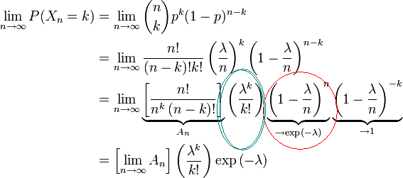
The two circled terms are the Poisson formula. I didn’t really realize how that red-circled part worked before. Look what it’s saying!
It is 1 – λ/n, which is the probability of NO event, ‘grown’ by the number of trials. In my examples above, I used events as opposed to probabilities of events. This makes no difference to the math, really, you just take the inverse of all your terms.
And now the code is clear: it just strings together a bunch of events until you hit the probability at which you know there can be no more events. And that probability is different when expressed a uniform distributed number than as an e-distributed number.
