Let me start with an easy example that everyone starts with in stats: we want to know how variable height is in the population of humans. We can’t measure the height of all humans so we gather up the few around us and here’s what we get.
Janet: 5ft
Sam: 6ft
Shaq: 7ft.
The average height of the three is: 
The variance of height is:
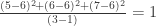
So the statistician says we now have an estimate for average height and variance of heights of the population of humans: 6ft tall with a variance of 1.
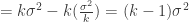
Here’s a twist, though. If there were only three humans in existence, the variance would be different: 
So what’s the difference? The difference is that if Janet, Sam and Shaq are a sample of the population we divide the sum of squared differences from the mean by n-1=2. If they are the entire population, we divide it by n=3. This makes the sample variance larger than the population variance. Why is that?
This is a question that annoyed me for some time. The key, though, is to not focus on the variance calculation. The key is the mean.
You see, when you pull out a sample of a population you aren’t measuring the correct average height. Your height estimate is going to be wrong and it’s going to be different each time you draw a sample from the population. In other words, it’s going to vary and so increase the variance.
So the point of the n-1 correction is to increase the variance estimate to allow for the fact that your measurement of the mean varies with each possible sample.
If the sample gets big enough, dividing by n-1 isn’t much different than dividing by n. Imagine the difference between dividing by 100,000 or 100,001. So this correction becomes meaningless because the mean we are measuring is probably the correct one.
Here’s the math:
Let’s start with the sum of squared errors, which is this: 


which is the same thing as saying this ![E[\frac{1}{(k-1)}\sum\limits_{j=1}^k(Y_j-\bar{Y})^2] = \sigma^2](https://s0.wp.com/latex.php?latex=E%5B%5Cfrac%7B1%7D%7B%28k-1%29%7D%5Csum%5Climits_%7Bj%3D1%7D%5Ek%28Y_j-%5Cbar%7BY%7D%29%5E2%5D+%3D+%5Csigma%5E2&bg=ffffff&fg=303030&s=0&c=20201002)
![= \sum\limits_{j=1}^k[(Y_j-\mu) + (\mu-\bar{Y})]^2](https://s0.wp.com/latex.php?latex=%3D+%5Csum%5Climits_%7Bj%3D1%7D%5Ek%5B%28Y_j-%5Cmu%29+%2B+%28%5Cmu-%5Cbar%7BY%7D%29%5D%5E2&bg=ffffff&fg=303030&s=0&c=20201002)
![= \sum\limits_{j=1}^k[(Y_j-\mu)^2 + 2(Y_j-\mu)(\mu-\bar{Y})+ (\mu-\bar{Y})^2]](https://s0.wp.com/latex.php?latex=%3D+%5Csum%5Climits_%7Bj%3D1%7D%5Ek%5B%28Y_j-%5Cmu%29%5E2+%2B+2%28Y_j-%5Cmu%29%28%5Cmu-%5Cbar%7BY%7D%29%2B+%28%5Cmu-%5Cbar%7BY%7D%29%5E2%5D&bg=ffffff&fg=303030&s=0&c=20201002)
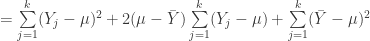
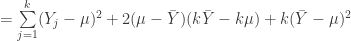
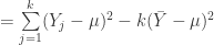
![E[\sum\limits_{j=1}^k(Y_j-\bar{Y})^2]](https://s0.wp.com/latex.php?latex=E%5B%5Csum%5Climits_%7Bj%3D1%7D%5Ek%28Y_j-%5Cbar%7BY%7D%29%5E2%5D&bg=ffffff&fg=303030&s=0&c=20201002)
![E[\sum\limits_{j=1}^k(Y_j-\mu)^2 -k(\bar{Y}-\mu)^2]](https://s0.wp.com/latex.php?latex=E%5B%5Csum%5Climits_%7Bj%3D1%7D%5Ek%28Y_j-%5Cmu%29%5E2+-k%28%5Cbar%7BY%7D-%5Cmu%29%5E2%5D&bg=ffffff&fg=303030&s=0&c=20201002)